Site Map
News and updates
| New releases and related tools will be announced through the mailing list |
Getting Help
| Questions about CummeRbund should be sent to lgoff@csail.mit.edu. |
Releases
Stable Version (tied to Bioconductor release cycle)
| version 2.0.0 (BioC 2.11) | 10/2/2012 |
| Package Source | |
| Mac OS X binary | |
| Windows binary |
Previous Releases
| version 1.2.0 (BioC 2.10) | 4/12/2012 |
* CummeRbund is now included as part of the R/Bioconductor project. The links above point to the R packages directly, and every effort should be made to use the version provided by Bioconductor as it will ensure compatibility with other Bioconductor packages. Easy installation instructions (with dependencies) can be found here.
Related Tools
Contributors
Links
v2.0.0 -- Oct 2, 2012
Contents
1 Requirements2 Introduction
3 CummeRbund Classes
3.1 CuffSet Class
3.2 CuffData Class
3.3 CuffDist Class
3.4 CuffFeatureSet Class
3.5 CuffFeature Class
4 Reading cuffdiff output
4.1 Adding additional feature annotation
5 Global statistics and Quality Control
6 Accessing Data
6.1 Writing your own SQL accessors
7 Creating Gene Sets
7.1 Geneset level plots
8 Individual Genes
8.1 Gene-level plots
8.1.1 Gene Feature plots
9 Data Exploration
9.1 Overview of significant features
9.2 Creating gene sets from significantly regulated genes
9.3 Exploring the relationships between conditions
9.3.1 Distance matrix
9.3.2 Dimensionality reduction
9.4 Partitioning
9.5 Specificity
9.6 Finding similar genes
10 Miscellaneous
11 Known Issues
12 Session info
1 Requirements
NOTE: cummeRbund 2.0 was designed in conjunction with the release of cufflinks 2.0. While we attempted to preserve backwards-compatability, it is highly recommended that you update your cufflinks version >=2.0 to take full advantage of the improvements in modeling, reporting, and visualization that have been incorporated.- Cufflinks ≥ v2.0.0
- SQLite
- R ≥ v2.7.0
- Packages:
- RSQLite
- ggplot2 v0.9.2
- reshape2
- plyr
- fastcluster
- rtracklayer
- Gviz
- BiocGenerics (>=0.3.2)
- Recommended:
- Hmisc
2 Introduction
cummeRbund is a visualization package for Cufflinks high-throughput sequencing data. It is designed to help you navigate through the large amount of data produced from a Cuffdiff RNA-Seq differential expression analysis. The results of this analysis are typically a large number of inter-related files that are not terribly intuitive to navigate through. cummeRbund helps promote rapid analysis of RNA-Seq data by aggregating, indexing, and allowing you easily visualize and create publication-ready figures of your RNA-Seq data while maintaining appropriate relationships between connected data points. CummeRbund is a multifaceted suite for streamlined analysis and visualization of massively parallel RNA differential expression data sequencing data. CummeRbund begins by re-organizing output files of a cuffdiff analysis, and storing these data in a local SQLite database. CummeRbund indexes the data to speed up access to specific feature data (genes, isoforms, TSS, CDS, etc.), and preserves the various relationships between these features. Access to data elements is managed via the RSQLite package and data are presented in appropriately structured R classes with various convenience functions designed to streamline your workflow. This persistent database storage means that inter-connected expression values are rapidly accessible and quickly searchable in future analyses. CummeRbund defines two types of data classes, 'pointer' or reference classes describe SQL connections to the database without directly containing data, and 'data' classes that retrieve a subset of related data points such as associated features from a given gene or gene set. Each class type has methods for direct access to FPKM vales, differential expression information, statistical test results, raw and normalized fragment counts, individual replicate FPKM values, and additional annotation information for features. Output formats allow for browsing and analysis of data in standard R objects (data.frame, list, etc). CummeRbund was designed to provide analysis and visualization tools analogous to microarray data. In this regard, numerous plotting methods are provided for visualization of RNA-Seq data quality and global statistics, and simple routines for plotting expression levels for one or thousands of genes, their isoforms, TSS groups, or CDS groups. The base class, cuffSet is a 'pointer' to cuffdiff data that are stored out-of-memory in a sqlite database.3 CummeRbund Classes
3.1 CuffSet Class
A pointer class to control access to the sqlite tables holding the Cufflinks data. The primary slot is DB which contains the RSQLite connection object. This can be accessed using the DB() accessor. The additional slots (genes, isoforms, TSS, and CDS) are each instances of the CuffData class and are pointers to sets of tables for each data subtype. They can be accessed with similar accessor wrappers. This is the default class created by readCufflinks. By default, CuffData accessor methods applied to a CuffSet class will operate on the 'genes' slot. The runInfo() method can be used to retrieve information about the actual cuffdiff run itself, including command-line arguments used to generate the results files.3.2 CuffData Class
The CuffData class is also a pointer class to the SQL backend, but each instance is specific for a data subtype (genes, isoforms, TSS, CDS). Again, there is an DB slot (accessible using DB()) that contains the RSQLite connection object. There are several accessor, setter, and plotting methods that allow for global analysis of all features within a CuffData class.Subsetting is currently being re-written, however, it is primarily done through the 'gene_id' field. Available slots for the CuffData class are:- DB: RSQLite connection object
- tables: A list of tables in the SQLite DB that contain the cufflinks data.
- filters: A list of filters for subsetting (not implemented yet).
- type: A character field describing the data (ie. 'genes','isoforms','TSS','CDS','other')
- idField: The name of the identifying index field for this object (eg. 'gene_id' for type='gene', or 'isoform_id' for type='isoform')
3.3 CuffDist Class
The CuffDist class is an pointer class that contains the results of the various 'distribution tests' performed by cuffdiff. These include differential promoter usage, differential splicing, and differential CDS usage. These are independent tests from the differential analysis of gene-, isoform-, TSS-, and CDS-level features and therefore have their own container type to distinguish them as such. The 'promoters', 'relCDS', and 'splicing' slots of a CuffSet class are all CuffDist instances. Available slots for the CuffDist class are:- DB: RSQLite connection object
- tables: A list of tables in the SQLite DB that contain the distribution test data.
- type: A character field describing the data (ie. 'promoters','relCDS','splicing')
- idField: The name of the identifying index field for this object (eg. 'TSS_group_id' for type='promoters', or 'CDS_id' for type='relCDS', etc.)
3.4 CuffFeatureSet Class
The CuffFeatureSet class is a data-storage container that holds all available data for a pre-determined list of features. Slots for FPKM data, differential regulation data, and feature-level annotation are all available. Unlike the previous classes, this class contains no connection information to the SQL database, but rather contains several slots with data.frame objects storing multiple-features worth of information. There are available accessors, and plotting methods that are designed to present multiple-features worth of information (eg. heatmaps, scatterplots, etc) Available slots for a CuffFeatureSet object include:- annotation: Holds all feature-level annotation information for all features in object.
- fpkm: A data frame of FPKM data across all conditions, for all features in object.
- repFpkm: A data frame of deconvolved FPKM values across individual replicates, for all features in object.
- diff: A data frame of differential expression/regulation data for all features in object.
- count: A data frame containing raw and normalized fragment counts, variance, dispersion, and uncertainty for all features in object.
- genome: A character string indicating which build of the genome the associated features are derived from. (e.g. `hg19',`mm9')
- ids: A 'character' list of all gene_ids used in object.
- isoforms: A CuffFeatureSet object for all isoforms of genes in object.
- TSS: A CuffFeatureSet object for all TSS of genes in object.
- CDS: A CuffFeatureSet object for all CDS of genes in object.
3.5 CuffFeature Class
The CuffFeature class is designed for single-feature-level data analysis and plotting. The methods available for this object are designed to analyze or visualize information about a specific feature. This is a 'data' object, as opposed to a 'pointer' object to the database backend. There is a validity requirement that a CuffFeature object only point to data from a single feature. Available slots for a CuffFeature object include:- annotation: Holds feature-level annotation information for a given feature.
- fpkm: A data frame of FPKM data across all samples for a given feature.
- repFpkm: A data frame of deconvolved FPKM values across all replicates for a given feature.
- diff: A data frame of differential expression/regulation data for a given feature.
- count: A data frame containing raw and normalized fragment counts, variance, dispersion, and uncertainty for a given feature.
- id: The common 'gene_id' for all data in object
- isoforms: A CuffFeature object for all isoforms of a given gene.
- TSS: A CuffFeature object for all TSS of a given gene.
- CDS: A CuffFeature object for all CDS of a given gene.
- features: A data.frame object containing feature information for the transcript models describing the gene.
4 Reading cuffdiff output
cummeRbund was designed to process the multi-file output format for a 'cuffdiff' differential expression analysis. In this type of analysis, a user will use a reference .gtf file (either known annotation or a .gtf file created from a cufflinks assembly or merge of assemblies) and quantitate the expression values and differential regulation of the annotation(s) in the .gtf file across two or more SAM/BAM files. By design, cuffdiff produces a number of output files that contain test results for changes in expression at the level of transcripts, primary transcripts, and genes. It also tracks changes in the relative abundance of transcripts sharing a common transcription start site, and in the relative abundances of the primary transcripts of each gene. Tracking the former allows one to see changes in splicing, and the latter lets one see changes in relative promoter use within a gene.Note:Early versions of Cuffdiff required that transcripts in the input GTF be annotated with certain attributes in order to look for changes in primary transcript expression, splicing, coding output, and promoter use. This is no longer the case with >=v1.1.1 of cummeRbund, however we still recommend the use of both the following attributes in your GTF file to enable all downstream features of cummeRbund.
These attributes are:
- tss_id: The ID of this transcript's inferred start site. Determines which primary transcript this processed transcript is believed to come from. Cuffcompare appends this attribute to every transcript reported in the .combined.gtf file.
- p_id The ID of the coding sequence this transcript contains. This attribute is attached by Cuffcompare to the .combined.gtf records only when it is run with a reference annotation that include CDS records. Further, differential CDS analysis is only performed when all isoforms of a gene have p_id attributes, because neither Cufflinks nor Cuffcompare attempt to assign an open reading frame to transcripts.
There are four FPKM tracking files:
- isoforms.fpkm_tracking Transcript FPKMs
- genes.fpkm_tracking Gene FPKMs. Tracks the summed FPKM of transcripts sharing each gene_id
- cds.fpkm_tracking Coding sequence FPKMs. Tracks the summed FPKM of transcripts sharing each p_id, independent of tss_id
- tss_groups.fpkm_tracking Primary transcript FPKMs. Tracks the summed FPKM of transcripts sharing each tss_id
Four .diff files are created:
- isoform_exp.diff Transcript differential FPKM.
- gene_exp.diff Gene differential FPKM. Tests difference sin the summed FPKM of transcripts sharing each gene_id
- tss_group_exp.diff Primary transcript differential FPKM. Tests differences in the summed FPKM of transcripts sharing each tss_id
- cds_exp.diff Coding sequence differential FPKM. Tests differences in the summed FPKM of transcripts sharing each p_id independent of tss_id
- splicing.diff Differential splicing tests.
- CDS.diff Differential coding output.
- promoters.diff Differential promoter use.
One of the principle benefits of using cummeRbund is that data are stored in a SQLite database. This allows for out-of-memory analysis of data, quick retrieval, and only a one-time cost to setup the tables. By default, cummeRbund assumes that all output files from cuffdiff are in the current working directory. To read these files, populate the 'cuffData.db' database backend, and return the CuffSet pointer object, you can do the following.
> library(cummeRbund)
> cuff<-readCufflinks()
> cuff
CuffSet instance with:
	 3 samples
	 400 genes
	 1203 isoforms
	 662 TSS
	 906 CDS
	 1062 promoters
	 1986 splicing
	 990 relCDS
Again, by default dir is assumed to be the current working directory and cuff<-readCufflinks() should work if all appropriate files are in the current working directory. We now also recommend that you use both the genome and gtfFile arguments to readCufflinks(). This will allow cummeRbund to archive the transcript structure information located in the .gtf file associated with your particular cuffdiff run, as well as associate these transcripts with an appropriate genome build (e.g. 'hg19', 'mm9', etc) so as to allow for transcript-level visualizations and future integration with other external resources. Should you need to rebuild the SQLite backend for any reason, you can add the option rebuild=T to readCufflinks. Once the database is created, readCufflinks will default to using the SQL backend and should not need to rebuild this database. Each R session should begin with a call to readCufflinks so as to initialize the database connection and create an object with the appropriate RSQLite connection information.
4.1 Adding additional feature annotation
Gene- or feature-level annotation can be permanently added to the database tables for future querying. If you have a data.frame where the first column contains the 'tracking_id' (eg. 'gene_id' for genes, 'isoform_id' for isoforms, etc). You can easily add feature level annotation using the addFeatures() function:
> annot<-read.table("gene_annotation.tab",sep="\t",header=T,na.string="-")
> addFeatures(cuff,annot,level="genes")
By default, features added to a CuffSet object are assumed to be gene-level annotations, but the level can selected using the argument level. Features added to a CuffData object are assumed to be of the same type as the 'type' value for that given object (e.g. gene-level features for 'genes', isoform-level features for isoforms, etc.)
5 Global statistics and Quality Control
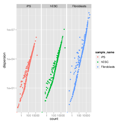
Several plotting methods are available that allow for quality-control or global analysis of cufflinks data. A good place to begin is to evaluate the quality of the model fitting. Overdispersion is a common problem in RNA-Seq data. As of cufflinks v2.0 mean counts, variance, and dispersion are all emitted, allowing you to visualize the estimated overdispersion for each sample as a quality control measure.> disp<-dispersionPlot(genes(cuff)) > disp
> genes.scv<-fpkmSCVPlot(genes(cuff))
> isoforms.scv<-fpkmSCVPlot(isoforms(cuff))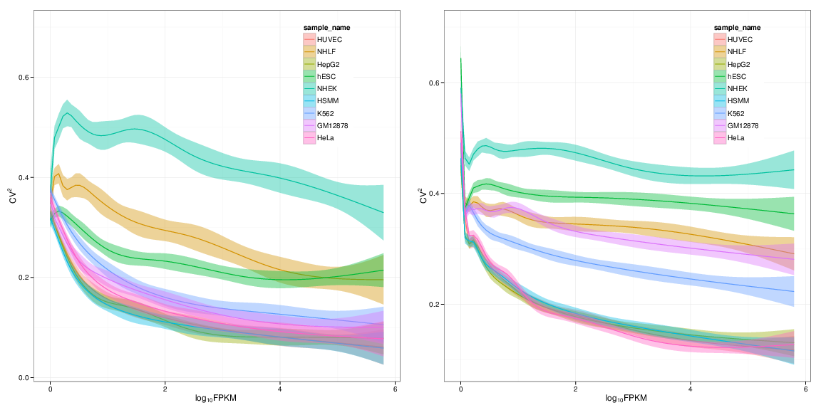
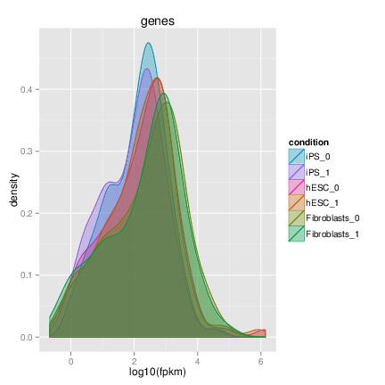
> dens<-csDensity(genes(cuff)) > dens> densRep<-csDensity(genes(cuff),replicates=T) > densRep
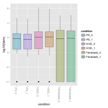
> b<-csBoxplot(genes(cuff)) > b> brep<-csBoxplot(genes(cuff),replicates=T) > brep
> s<-csScatterMatrix(genes(cuff))
> s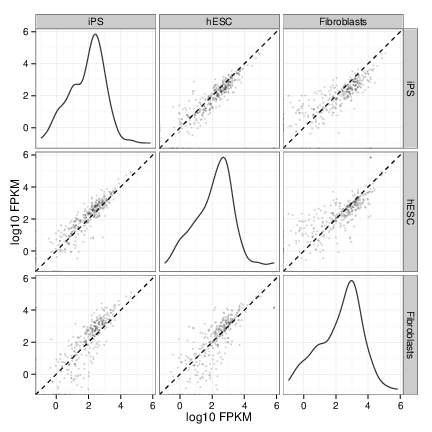
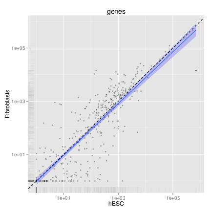
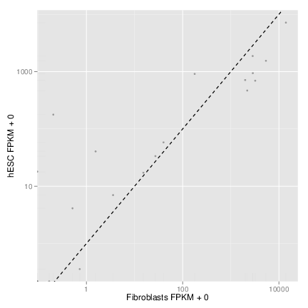
> s<-csScatter(genes(cuff),"hESC","Fibroblasts",smooth=T)
> s
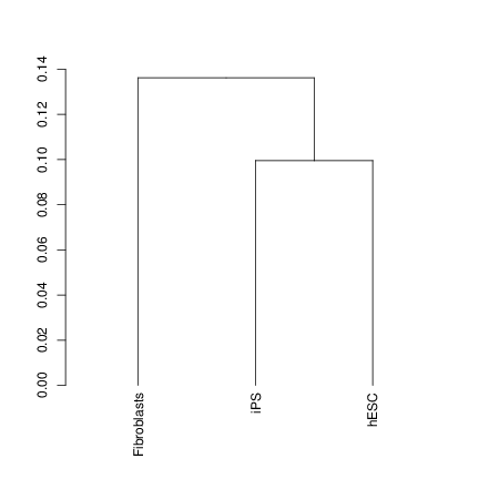
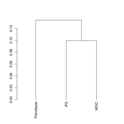
> dend<-csDendro(genes(cuff))
> dend
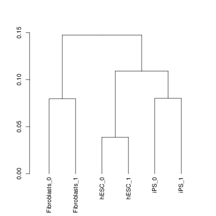
 > dend.rep<-csDendro(genes(cuff),replicates=T)
> dend.rep
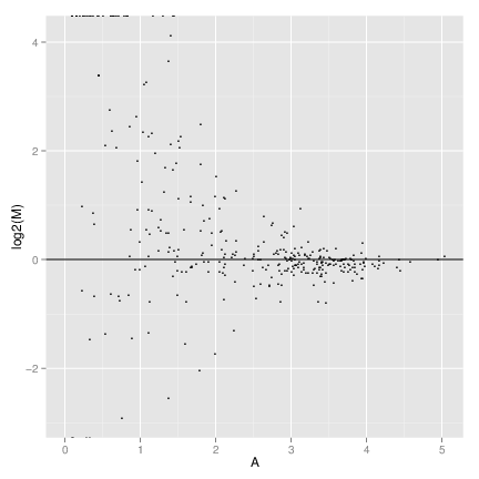
> m<-MAplot(genes(cuff),"hESC","Fibroblasts") > m> mCount<-MAplot(genes(cuff),"hESC","Fibroblasts",useCount=T) > mCount
> v<-csVolcanoMatrix(genes(cuff))
> v
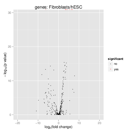
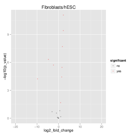
> v<-csVolcano(genes(cuff),"hESC","Fibroblasts")
> v
6 Accessing Data
Cuffdiff run information
Run-level information such as run parameters, and sample information can be accessed from a CuffSet object by using the runInfo and replicates methods:> runInfo(cuff)
          param
1      cmd_line
2       version
3  SVN_revision
4 boost_version
5        genome
                                                                                                                                                    value
1 cuffdiff -L iPS,hESC,Fibroblasts -p 6 chr1_snippet.gtf -o iPS_hESC_fibro iPS_rep1.bam,iPS_rep2.bam H1_rep1.bam,H1_rep3.bam NHLF_rep1.bam,NHLF_rep2.bam
2                                                                                                                                                   1.4.0
3                                                                                                                                                    3285
4                                                                                                                                                  104900
5                                                                                                                                                    hg19
> replicates(cuff)
           file sample_name replicate      rep_name total_mass
1  iPS_rep1.bam         iPS         0         iPS_0     173431
2  iPS_rep2.bam         iPS         1         iPS_1     173007
3   H1_rep1.bam        hESC         0        hESC_0     754749
4   H1_rep3.bam        hESC         1        hESC_1     762643
5 NHLF_rep1.bam Fibroblasts         0 Fibroblasts_0     876775
6 NHLF_rep2.bam Fibroblasts         1 Fibroblasts_1    1412130
  norm_mass internal_scale external_scale
1    706934       0.958068       0.584877
2    706934       1.037970       0.584877
3    706934       0.989851       1.513060
4    706934       1.010250       1.513060
5    706934       0.840416       1.223240
6    706934       1.198470       1.223240
Features/Annotation
Feature-level information can be accessed directly from a CuffData object using the fpkm, repFpkm, count, diffData, or annotation methods:> gene.features<-annotation(genes(cuff)) > head(gene.features)
      gene_id class_code nearest_ref_id gene_short_name
1 XLOC_000001       <NA>           <NA>            <NA>
2 XLOC_000002       <NA>           <NA>           OR4F5
3 XLOC_000003       <NA>           <NA>            <NA>
4 XLOC_000004       <NA>           <NA>            <NA>
5 XLOC_000005       <NA>           <NA>            <NA>
6 XLOC_000006       <NA>           <NA>          OR4F16
               locus length coverage
1   chr1:11873-29961     NA       NA
2   chr1:69090-70008     NA       NA
3 chr1:321083-321114     NA       NA
4 chr1:321145-321223     NA       NA
5 chr1:322036-328580     NA       NA
6 chr1:367658-368595     NA       NA
> gene.fpkm<-fpkm(genes(cuff))
> head(gene.fpkm)
      gene_id sample_name       fpkm    conf_hi conf_lo
1 XLOC_000001 Fibroblasts    16.1506   182.9240 0.00000
2 XLOC_000002 Fibroblasts     0.0000     0.0000 0.00000
3 XLOC_000003 Fibroblasts     0.0000     0.0000 0.00000
4 XLOC_000004 Fibroblasts 14237.7000 78180.9000 0.00000
5 XLOC_000005 Fibroblasts    48.0566    90.6526 5.46055
6 XLOC_000006 Fibroblasts     0.0000     0.0000 0.00000
  quant_status      stdev
1           OK    83.3867
2           OK     0.0000
3           OK     0.0000
4           OK 31971.6000
5           OK    21.2980
6           OK     0.0000
> gene.repFpkm<-repFpkm(genes(cuff))
> head(gene.repFpkm)
      gene_id sample_name replicate      rep_name  raw_frags
1 XLOC_000001 Fibroblasts         0 Fibroblasts_0  12.000100
2 XLOC_000002 Fibroblasts         0 Fibroblasts_0   0.000000
3 XLOC_000003 Fibroblasts         0 Fibroblasts_0   0.000000
4 XLOC_000004 Fibroblasts         0 Fibroblasts_0   0.333333
5 XLOC_000005 Fibroblasts         0 Fibroblasts_0 137.100000
6 XLOC_000006 Fibroblasts         0 Fibroblasts_0   0.000000
  internal_scaled_frags external_scaled_frags       fpkm
1             14.278800             11.672900    11.1815
2              0.000000              0.000000     0.0000
3              0.000000              0.000000     0.0000
4              0.396629              0.324245 28475.5000
5            163.134000            133.362000    57.8929
6              0.000000              0.000000     0.0000
  effective_length status
1               NA     OK
2               NA     OK
3               NA     OK
4               NA     OK
5               NA     OK
6               NA     OK
> gene.counts<-count(genes(cuff))
> head(gene.counts)
      gene_id sample_name      count    variance uncertainty
1 XLOC_000001 Fibroblasts  20.072500 1.05160e+04 1.77636e-15
2 XLOC_000002 Fibroblasts   0.000000 0.00000e+00 0.00000e+00
3 XLOC_000003 Fibroblasts   0.000000 0.00000e+00 0.00000e+00
4 XLOC_000004 Fibroblasts   0.198315 1.98315e-01 0.00000e+00
5 XLOC_000005 Fibroblasts 131.575000 3.35882e+03 5.68434e-14
6 XLOC_000006 Fibroblasts   0.000000 0.00000e+00 0.00000e+00
   dispersion status
1 1311.870000     OK
2    0.000000     OK
3    0.000000     OK
4    0.198315     OK
5 2161.890000     OK
6    0.000000     OK
> isoform.fpkm<-fpkm(isoforms(cuff))
> head(isoform.fpkm)
      isoform_id sample_name        fpkm   conf_hi conf_lo
1 TCONS_00000001 Fibroblasts    10.99630   118.178       0
2 TCONS_00000002 Fibroblasts     0.00000     0.000       0
3 TCONS_00000003 Fibroblasts     5.15434   132.926       0
4 TCONS_00000004 Fibroblasts     0.00000     0.000       0
5 TCONS_00000005 Fibroblasts     0.00000     0.000       0
6 TCONS_00000006 Fibroblasts 14237.70000 78180.900       0
  quant_status       stdev
1           OK    53.59085
2           OK     0.00000
3           OK    63.88583
4           OK     0.00000
5           OK     0.00000
6           OK 31971.60000
> gene.diff<-diffData(genes(cuff))
> head(gene.diff)
      gene_id sample_1 sample_2 status   value_1     value_2
1 XLOC_000001      iPS     hESC NOTEST  20.21750 3.47386e-01
2 XLOC_000002      iPS     hESC NOTEST   0.00000 0.00000e+00
3 XLOC_000003      iPS     hESC NOTEST   0.00000 0.00000e+00
4 XLOC_000004      iPS     hESC     OK   0.00000 6.97259e+05
5 XLOC_000005      iPS     hESC     OK 355.82300 6.96704e+02
6 XLOC_000006      iPS     hESC NOTEST   1.51396 0.00000e+00
  log2_fold_change     test_stat    p_value    q_value
1     -5.86292e+00   7.13525e-01 0.47552100 1.00000000
2      0.00000e+00   0.00000e+00 1.00000000 1.00000000
3      0.00000e+00   0.00000e+00 1.00000000 1.00000000
4     1.79769e+308  1.79769e+308 0.00857693 0.02109120
5      9.69385e-01  -2.98373e+00 0.00284757 0.00840284
6    -1.79769e+308 -1.79769e+308 0.24382400 1.00000000
  significant
1          no
2          no
3          no
4         yes
5         yes
6          no
Condition and feature names
Vectors of sample names and feature names are available by using the samples and featureNames methods:> sample.names<-samples(genes(cuff)) > head(sample.names)
[1] "iPS" "hESC" "Fibroblasts"
> gene.featurenames<-featureNames(genes(cuff))
> head(gene.featurenames)
[1] "XLOC_000001" "XLOC_000002" "XLOC_000003" "XLOC_000004"
[5] "XLOC_000005" "XLOC_000006"
Convenience functions
To facilitate Bioconductor-like operations, an 'FPKM-matrix' can be returned easily using the fpkmMatrix method:> gene.matrix<-fpkmMatrix(genes(cuff)) > head(gene.matrix)
                  iPS        hESC Fibroblasts
XLOC_000001  20.21750 3.47386e-01     16.1506
XLOC_000002   0.00000 0.00000e+00      0.0000
XLOC_000003   0.00000 0.00000e+00      0.0000
XLOC_000004   0.00000 6.97259e+05  14237.7000
XLOC_000005 355.82300 6.96704e+02     48.0566
XLOC_000006   1.51396 0.00000e+00      0.0000
A matrix of replicate FPKM values can be retrieved by using repFpkmMatrix
> gene.rep.matrix<-repFpkmMatrix(genes(cuff))
> head(gene.rep.matrix)
               iPS_0     iPS_1      hESC_0      hESC_1
XLOC_000001  17.2049  22.92880       0.000 6.21918e-01
XLOC_000002   0.0000   0.00000       0.000 0.00000e+00
XLOC_000003   0.0000   0.00000       0.000 0.00000e+00
XLOC_000004   0.0000   0.00000 1377990.000 8.35811e+05
XLOC_000005 319.0300 390.45500     687.563 7.21983e+02
XLOC_000006   0.0000   3.02791       0.000 0.00000e+00
            Fibroblasts_0 Fibroblasts_1
XLOC_000001       11.1815       20.6009
XLOC_000002        0.0000        0.0000
XLOC_000003        0.0000        0.0000
XLOC_000004    28475.5000        0.0000
XLOC_000005       57.8929       38.0084
XLOC_000006        0.0000        0.0000
Similarly, a matrix of normalized counts can be generated by using countMatrix
> gene.count.matrix<-countMatrix(genes(cuff))
> head(gene.count.matrix)
                   iPS        hESC Fibroblasts
XLOC_000001  11.440900    0.494996   20.072500
XLOC_000002   0.000000    0.000000    0.000000
XLOC_000003   0.000000    0.000000    0.000000
XLOC_000004   0.000000    5.680560    0.198315
XLOC_000005 486.456000 2495.560000  131.575000
XLOC_000006   0.481711    0.000000    0.000000
6.1 Writing your own SQL accessors
Since the cuffData.db is a SQLite database backend, if you are familiar with SQL and/or RSQLite query construction, you can simply design your own SQL queries to access the data that you are after.7 Creating Gene Sets
Gene Sets (stored in a CuffGeneSet object) can be created using the getGenes method on a CuffSet object. You must first create a vector of 'gene_id' or 'gene_short_name' values to identify the genes you wish to select:> data(sampleData) > myGeneIds<-sampleIDs > myGeneIds
 [1] "XLOC_001363" "XLOC_001297" "XLOC_001339" "XLOC_000132"
 [5] "XLOC_001265" "XLOC_000151" "XLOC_001359" "XLOC_000069"
 [9] "XLOC_000170" "XLOC_000105" "XLOC_001262" "XLOC_001348"
[13] "XLOC_001411" "XLOC_001369" "XLOC_000158" "XLOC_001370"
[17] "XLOC_001263" "XLOC_000115" "XLOC_000089" "XLOC_001240"
> myGenes<-getGenes(cuff,myGeneIds)
> myGenes
CuffGeneSet instance for  20  genes

Slots:
	 annotation
	 fpkm
	 repFpkm
	 diff
	 count
	 isoforms	 CuffFeatureSet instance of size 45
	 TSS		 CuffFeatureSet instance of size 23
	 CDS		 CuffFeatureSet instance of size 36
	 promoters		 CuffFeatureSet instance of size 20
	 splicing		 CuffFeatureSet instance of size 23
	 relCDS		 CuffFeatureSet instance of size 20
The same fpkm, repFpkm, count, annotation, diffData, samples, and featureNames methods are available for instances of the CuffGeneSet class, but additional accessor methods are available for the promoters, relCDS, and splicing slot data as well.
> #FPKM values for genes in gene set
> head(fpkm(myGenes))
      gene_id sample_name        fpkm     conf_hi  conf_lo
1 XLOC_000069 Fibroblasts 2.05083e-01 8.94501e-01    0.000
2 XLOC_000069        hESC 1.77686e+02 2.15888e+02  139.484
3 XLOC_000069         iPS 1.90000e+01 3.88149e+01    0.000
4 XLOC_000089 Fibroblasts 1.39701e+04 2.19187e+04 6021.450
5 XLOC_000089        hESC 7.18339e+03 7.92296e+03 6443.810
6 XLOC_000089         iPS 1.41690e+03 1.96558e+03  868.215
  quant_status       stdev
1           OK    0.344709
2           OK   19.101000
3           OK    9.907450
4           OK 3974.300000
5           OK  369.785000
6           OK  274.340000
> #Isoform-level FPKMs for gene set
> head(fpkm(isoforms(myGenes)))
      isoform_id sample_name       fpkm    conf_hi   conf_lo
1 TCONS_00000179 Fibroblasts   0.205083   0.894501   0.00000
2 TCONS_00000179        hESC  20.360900  33.840500   6.88119
3 TCONS_00000179         iPS   7.694340  16.356900   0.00000
4 TCONS_00000180 Fibroblasts   0.000000   0.000000   0.00000
5 TCONS_00000180        hESC 157.325000 198.673000 115.97800
6 TCONS_00000180         iPS  11.305600  27.105700   0.00000
  quant_status     stdev
1           OK  0.344709
2           OK  6.739800
3           OK  4.331280
4           OK  0.000000
5           OK 20.674000
6           OK  7.900050
> #Replicate FPKMs for TSS groups within gene set
> head(repFpkm(TSS(myGenes)))
  TSS_group_id sample_name replicate      rep_name raw_frags
1       TSS128         iPS         0         iPS_0     987.0
2       TSS128         iPS         1         iPS_1    1065.0
3       TSS128        hESC         1        hESC_1   13196.0
4       TSS128        hESC         0        hESC_0   13588.0
5       TSS128 Fibroblasts         1 Fibroblasts_1   18899.5
6       TSS128 Fibroblasts         0 Fibroblasts_0   22201.0
  internal_scaled_frags external_scaled_frags     fpkm
1               1030.20               1761.39  1412.22
2               1026.04               1754.29  1404.74
3              13062.10               8632.91  7131.86
4              13727.30               9072.58  7500.15
5              15769.70              12891.80 10368.60
6              26416.70              21595.70 17372.90
  effective_length status
1               NA     OK
2               NA     OK
3               NA     OK
4               NA     OK
5               NA     OK
6               NA     OK
>As of cummeRbund v2.0 CuffGeneSet classes can be created from any type of identifier ('gene_id','isoform_id','TSS_group_id', or 'CDS_id'). When you pass a list of identifiers that are not gene_id to getGenes(), the function attempts to lookup the parent gene_id for each feature and returns all relevant information for the given genes and all of their sub-features (not just the sub-features passed to getGenes()). If you are interested in just retrieving information for a given set of features, please use the new getFeatures() method described later.
7.1 Geneset level plots
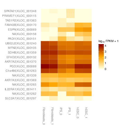
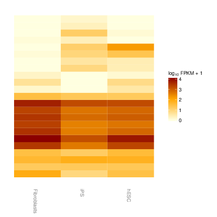
There are several plotting functions available for gene-set-level visualization: The csHeatmap() function is a plotting wrapper that takes as input either a CuffGeneSet or a CuffFeatureSet object (essentially a collection of genes and/or features) and produces a heatmap of FPKM expression values. The 'cluster' argument can be used to re-order either 'row', 'column', or 'both' dimensions of this matrix. By default, the Jensen-Shannon distance is used as the clustering metric, however, any function that produces a dist object can be passed to the 'cluster' argument as well.> h<-csHeatmap(myGenes,cluster='both') > h> h.rep<-csHeatmap(myGenes,cluster='both',replicates=T) > h.rep
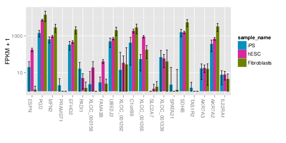
> b<-expressionBarplot(myGenes)
> b
> s<-csScatter(myGenes,"Fibroblasts","hESC",smooth=T)
> s
> v<-csVolcano(myGenes,"Fibroblasts","hESC")
> v
> ih<-csHeatmap(isoforms(myGenes),cluster='both',labRow=F) > ih> th<-csHeatmap(TSS(myGenes),cluster='both',labRow=F) > th
> den<-csDendro(myGenes)
8 Individual Genes
An individual CuffGene object can be created by using the getGene() function for a given 'gene_id' or 'gene_short_name'. As of cummeRbund ≥ v2.0 you can also use isoform_id, tss_group_id, or cds_id values to retrieve the corresponding parent gene object.> myGeneId<-"PINK1" > myGene<-getGene(cuff,myGeneId) > myGene
CuffGene instance for gene XLOC_000172
Short name:	 PINK1
Slots:
	 annotation
	 features
	 fpkm
	 repFpkm
	 diff
	 count
	 isoforms	 CuffFeature instance of size 2
	 TSS		 CuffFeature instance of size 2
	 CDS		 CuffFeature instance of size 2
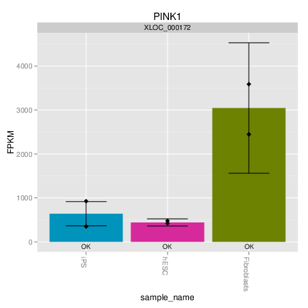
> head(fpkm(myGene))
      gene_id sample_name     fpkm  conf_hi  conf_lo
1 XLOC_000172 Fibroblasts 3045.930 4529.840 1562.020
2 XLOC_000172        hESC  441.939  523.916  359.961
3 XLOC_000172         iPS  640.208  914.562  365.853
  quant_status
1           OK
2           OK
3           OK
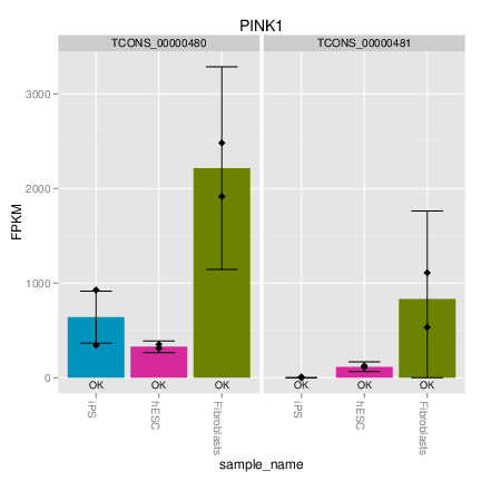
> head(fpkm(isoforms(myGene)))
      isoform_id sample_name     fpkm  conf_hi   conf_lo
1 TCONS_00000480 Fibroblasts 2213.850 3284.980 1142.7100
2 TCONS_00000480        hESC  326.979  388.108  265.8500
3 TCONS_00000480         iPS  640.208  914.562  365.8530
4 TCONS_00000481 Fibroblasts  832.083 1760.820    0.0000
5 TCONS_00000481        hESC  114.960  166.530   63.3891
6 TCONS_00000481         iPS    0.000    0.000    0.0000
  quant_status
1           OK
2           OK
3           OK
4           OK
5           OK
6           OK
8.1 Gene-level plots
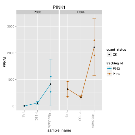
> gl<-expressionPlot(myGene) > gl> gl.rep<-expressionPlot(myGene,replicates=TRUE) > gl.rep
> gl.iso.rep<-expressionPlot(isoforms(myGene),replicates=T) > gl.iso.rep
> gl.cds.rep<-expressionPlot(CDS(myGene),replicates=T) > gl.cds.rep
> gb<-expressionBarplot(myGene) > gb> gb.rep<-expressionBarplot(myGene,replicates=T) > gb.rep
> igb<-expressionBarplot(isoforms(myGene),replicates=T)
> igb
8.1.1 Gene Feature plots
If you included both the genome build and gtfFile in your call to readCufflinks() then you will be able to access some of the transcript-structure level features that are now being integrated into cummeRbund. For now, these features are extended only to the single gene, CuffGene objects. Feature data are loaded into the \'features\'table of the cuffData.db database. When a CuffGene object is created using getGene(), all relative features are selected from this table and a \'features\'slot is added to the resulting object.> head(features(myGene))
  seqnames    start      end width strand source type score
1     chr1 20959948 20960428   481      + coding exon    NA
2     chr1 20964335 20964622   288      + coding exon    NA
3     chr1 20966385 20966485   101      + coding exon    NA
4     chr1 20970983 20971165   183      + coding exon    NA
5     chr1 20972053 20972216   164      + coding exon    NA
6     chr1 20974998 20975125   128      + coding exon    NA
  phase class_code exon_number     gene_id gene_name nearest_ref
1    NA          =           1 XLOC_000172     PINK1  uc001bdm.2
2    NA          =           2 XLOC_000172     PINK1  uc001bdm.2
3    NA          =           3 XLOC_000172     PINK1  uc001bdm.2
4    NA          =           4 XLOC_000172     PINK1  uc001bdm.2
5    NA          =           5 XLOC_000172     PINK1  uc001bdm.2
6    NA          =           6 XLOC_000172     PINK1  uc001bdm.2
         oId CDS_id     isoform_id TSS_group_id
1 uc001bdm.2   P364 TCONS_00000480       TSS264
2 uc001bdm.2   P364 TCONS_00000480       TSS264
3 uc001bdm.2   P364 TCONS_00000480       TSS264
4 uc001bdm.2   P364 TCONS_00000480       TSS264
5 uc001bdm.2   P364 TCONS_00000480       TSS264
6 uc001bdm.2   P364 TCONS_00000480       TSS264
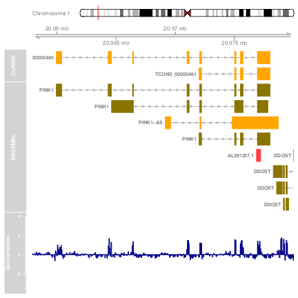
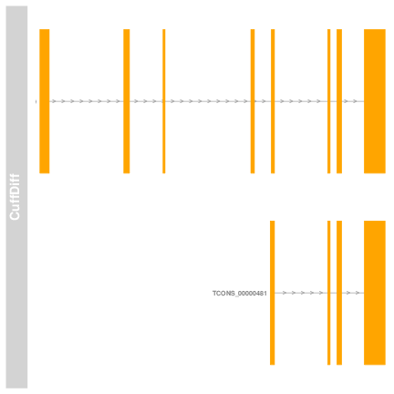
The Gviz package can be used to display features in a 'track'-like format. In particular, the GeneRegionTrack class creates a mechanism by which we can start to visualize transcript-level structures in their genomic context. cummeRbund implements the makeGeneRegionTrack() method to quickly create a GeneRegionTrack from the gene features.
> genetrack<-makeGeneRegionTrack(myGene)
> plotTracks(genetrack)
 We can then use some of the additional features from the Gviz package
to add additional tracks from an external data source.
> trackList<-list()
> myStart<-min(features(myGene)$start)
> myEnd<-max(features(myGene)$end)
> myChr<-unique(features(myGene)$seqnames)
> genome<-'hg19'
> ideoTrack <- IdeogramTrack(genome = genome, chromosome = myChr)
> trackList<-c(trackList,ideoTrack)
> axtrack<-GenomeAxisTrack()
> trackList<-c(trackList,axtrack)
> genetrack<-makeGeneRegionTrack(myGene)
> genetrack
GeneRegionTrack 'CuffDiff'
| genome: hg19
| active chromosome: chr1
| annotation features: 12
> trackList<-c(trackList,genetrack)
> biomTrack<-BiomartGeneRegionTrack(genome=genome,chromosome=as.character(myChr),
+ 		start=myStart,end=myEnd,name="ENSEMBL",showId=T)
> trackList<-c(trackList,biomTrack)
> conservation <- UcscTrack(genome = genome, chromosome = myChr,
+ 		track = "Conservation", table = "phyloP46wayPlacental",
+ 		from = myStart-2000, to = myEnd+2000, trackType = "DataTrack",
+ 		start = "start", end = "end", data = "score",
+ 		type = "hist", window = "auto", col.histogram = "darkblue",
+ 		fill.histogram = "darkblue", ylim = c(-3.7, 4),
+ 		name = "Conservation")
> trackList<-c(trackList,conservation)
> plotTracks(trackList,from=myStart-2000,to=myEnd+2000)
>
9 Data Exploration
The cummeRbund package is more than just a visualization tool as well. We are working to implement several different means of data exploration from gene and condition clustering, finding features with similar expression profiles, as well as incorporating Gene Ontology analysis.9.1 Overview of significant features
The sigMatrix() function can provide you with a "quick-and-dirty" view of the number of significant features of a particular type, and at a given alpha (0.05 by default). For example:> mySigMat<-sigMatrix(cuff,level='genes',alpha=0.05) > mySigMat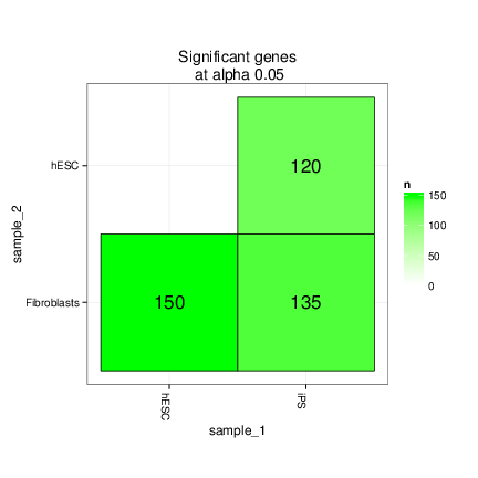
9.2 Creating gene sets from significantly regulated genes
One of the primary roles of a differential expression analysis is to conduct significance tests on each feature (genes, isoforms, TSS, and CDS) for appropriate pairwise comparisons of conditions. The results of these tests (after multiple testing correction of course) can be used to determine which genes are differentially regulated. cummeRbund makes accessing the results of these significance tests simple via getSig(). This function takes a CuffSet object and will scan at various feature levels ('genes' by default) to produce a vector of feature IDs. By default getSig() outputs a vector of tracking IDs corresponding to all genes that reject the null hypothesis in any condition tested. The default feature type can be changed by adjusting the 'level' argument to getSig(). In addition, a alpha value can be provided on which to filter the resulting list (the default is 0.05 to match the default of cuffdiff).> mySigGeneIds<-getSig(cuff,alpha=0.05,level='genes') > head(mySigGeneIds)
[1] "XLOC_000004" "XLOC_000005" "XLOC_000008" "XLOC_000009"
[5] "XLOC_000011" "XLOC_000013"
> length(mySigGeneIds)
[1] 207By default getSig() outputs a vector of tracking IDs corresponding to all genes that reject the null hypothesis in any condition tested. The default feature type can be changed by adjusting the 'level' argument to getSig(). In addition, a alpha value can be provided on which to filter the resulting list (the default is 0.05 to match the default of cuffdiff). Significance results for specific pairwise comparisons can be retrieved as well by specifying the two conditions as 'x' and 'y'. In this case, p-values are adjusted to reduce the impact of multiple-testing correction when only one set of tests is being conducted.
> hESC_vs_iPS.sigIsoformIds<-getSig(cuff,x='hESC',y='iPS',alpha=0.05,level='isoforms')
> head(hESC_vs_iPS.sigIsoformIds)
[1] "TCONS_00000006" "TCONS_00000013" "TCONS_00000015"
[4] "TCONS_00000018" "TCONS_00000034" "TCONS_00000041"
> length(hESC_vs_iPS.sigIsoformIds)
[1] 118The values returned for each level of this list can be used as an argument to getGenes, to create a CuffGeneSet object of significantly regulated genes (or features).
> mySigGenes<-getGenes(cuff,mySigGeneIds)
> mySigGenes
CuffGeneSet instance for  207  genes

Slots:
	 annotation
	 fpkm
	 repFpkm
	 diff
	 count
	 isoforms	 CuffFeatureSet instance of size 717
	 TSS		 CuffFeatureSet instance of size 399
	 CDS		 CuffFeatureSet instance of size 577
	 promoters		 CuffFeatureSet instance of size 207
	 splicing		 CuffFeatureSet instance of size 399
	 relCDS		 CuffFeatureSet instance of size 207
>Alternatively, you can use the getSigTable() method to return a full test-table of 'significant features' x 'pairwise tests' for all comparisons. Only features in which the null hypothesis can be rejected in at least one test are reported.
> mySigTable<-getSigTable(cuff,alpha=0.01,level='genes')
> head(mySigTable,20)
            hESCvsFibroblasts iPSvsFibroblasts iPSvshESC
XLOC_000005                 1                1         1
XLOC_000008                 0                1         1
XLOC_000009                 1                1         1
XLOC_000011                 0                1         1
XLOC_000013                 0                1         0
XLOC_000014                 1               NA         0
XLOC_000016                 0                0         1
XLOC_000017                 0                1         0
XLOC_000018                 1                1         0
XLOC_000019                 0                1         1
XLOC_000025                 1               NA         1
XLOC_000026                 1                1         0
XLOC_000027                 0                1         1
XLOC_000029                 1                1         0
XLOC_000032                 1               NA         0
XLOC_000034                 1                0         1
XLOC_000036                 0                1         1
XLOC_000044                 1               NA         1
XLOC_000047                 1                1         1
XLOC_000048                 1                1         0
9.3 Exploring the relationships between conditions
9.3.1 Distance matrix
Similarities between conditions and/or replicates can provide useful insight into the relationship between various groupings of conditions and can aid in identifying outlier replicates that do not behave as expected. cummeRbund provides the csDistHeat() method to visualize the pairwise similarities between conditions:> myDistHeat<-csDistHeat(genes(cuff)) > myDistHeat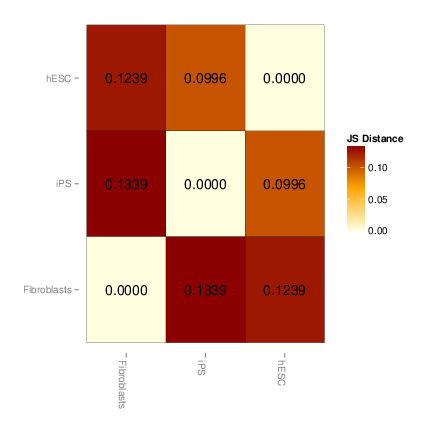
> myRepDistHeat<-csDistHeat(genes(cuff),replicates=T)
> myRepDistHeat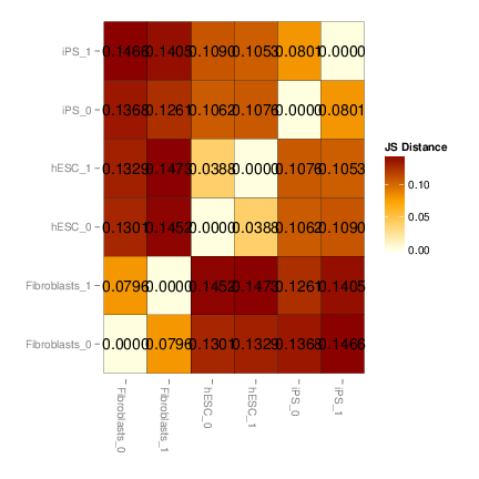
9.3.2 Dimensionality reduction
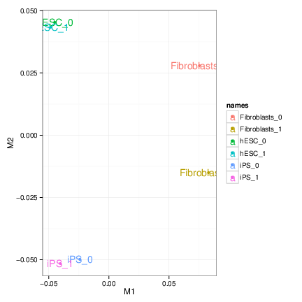
Dimensionality reduction is an informative approach for clustering and exploring the relationships between conditions. It can be useful for feature selection as well as identifying the sources of variability within your data. To this end, we have applied two different dimensionality reduction strategies in cummeRbund: principal component analysis (PCA) and multi-dimensional scaling (MDS). We provide the two wrapper methods, PCAplot and MDSplot> genes.PCA<-PCAplot(genes(cuff),"PC1","PC2") > genes.PCA> genes.MDS<-MDSplot(genes(cuff)) > genes.MDS
> genes.PCA.rep<-PCAplot(genes(cuff),"PC1","PC2",replicates=T) > genes.PCA.rep
> genes.MDS.rep<-MDSplot(genes(cuff),replicates=T) > genes.MDS.rep
9.4 Partitioning
K-means clustering is a useful tool that can be helpful in identifying clusters of genes with similar expression profiles. In fact, these profiles are learned from the data during the clustering. csCluster() uses the pam() method from the clustering package to perform the partitioning around medoids. In this case however, the distance metric used by default is the Jensen-Shannon distance instead of the default Euclidean distance. Prior to performing this particular partitioning, the user must choose the number of clusters (K) into which the expression profiles should be divided.> ic<-csCluster(myGenes,k=4) > head(ic$cluster)
XLOC_000069 XLOC_000089 XLOC_000105 XLOC_000115 XLOC_000132
          1           2           2           3           2
XLOC_000151
          1
> icp<-csClusterPlot(ic)
> icp
As of v1.1.1 of cummeRbund, the output of csCluster is a modified pam object. This replaces the default plotting behavior of the original csCluster plot to allow for further analysis of the clustering results. The original plotting behavior has been recapitulated in the csClusterPlot() method.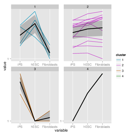
9.5 Specificity
In some cases, a researcher may be interested in identifying features that are 'condition-specific'. Or, more likely, producing an ordered list of genes based on their specificity for a given condition. We define a specificity score (S) as the following:
| (1) |
> myGenes.spec<-csSpecificity(myGenes)
> head(myGenes.spec)
             iPS_spec hESC_spec Fibroblasts_spec
XLOC_000069 0.6381500 0.7411063        0.4730055
XLOC_000089 0.6073556 0.6332403        0.6435982
XLOC_000105 0.6163066 0.6235261        0.6445646
XLOC_000115 1.0000000 0.4513380        0.4513380
XLOC_000132 0.6126800 0.6199645        0.6514962
XLOC_000151 0.7244614 0.6295328        0.5141304
S=1.0 if the feature is expressed exclusively in that condition. The findSimilar() method outlined below is another method that can be used to identify genes based on specificity but has the added feature that you can determine similarity to a more complex q expression profile.
9.6 Finding similar genes
Another common question in large-scale gene expression analyses is 'How can I find genes with similar expression profiles to gene x?'. We have implemented a method, findSimilar to allow you to identify a fixed number of the most similar genes to a given gene of interest. For example, if you wanted to find the 20 genes most similar to "PINK1", you could do the following:> mySimilar<-findSimilar(cuff,"PINK1",n=20) > mySimilar.expression<-expressionPlot(mySimilar,logMode=T,showErrorbars=F) > mySimilar.expression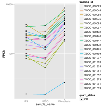
- If 'returnGeneSet' is set to FALSE, then findSimilar returns a data.frame of distance-ranked similar genes with distances. This is useful if you would like to see a rank-ordered list of similar genes.
- The 'distThresh' argument allows you to pass a value [between 0-1] to be used as a distance threshold instead of an arbitrary 'n' number of genes. setting distThresh=1.0 will return all genes ranked by their distance to your gene of interest.
> myProfile<-c(500,0,400)
> mySimilar2<-findSimilar(cuff,myProfile,n=10)
> mySimilar2.expression<-expressionPlot(mySimilar2,logMode=T,showErrorbars=F)
> mySimilar2.expression

10 Miscellaneous
- In appropriate plots, using the argument replicates=T will allow you to visualize replicate-level FPKM values either in lieu of or in addition to condition-level FPKMs.
- As of v1.1.3 we attempt to provide new visual cues in most plots that will indicate the quantification status for a particular feature in each given condition. We have enabled this feature by default for most plots to suggest a measure of reliability for each feature in a particular condition. In most cases, this feature can be disabled by setting 'showStatus=FALSE'.
- CummeRbund will now work with the hidden '-no-diff' argument for cuffdiff. This will quantify features against .bam files but not do differential testing. This is useful when you want to aggregate very large numbers of conditions, and cannot afford the time or space for the differential test results. (Not recommended unless you have a SPECIFIC need for this).
- All plotting functions return ggplot objects and the resulting objects can be manipulated/faceted/altered using standard ggplot2 methods.
- There are occasional DB connectivity issues that arise. Not entirely sure why yet. If necessary, just readCufflinks again and this should solve connectivity issues with a new RSQLite connection object. If connectivity continues to be a problem, try cuff<-readCufflinks(rebuild=T)
- I am still working on fully documenting each of the methods. There are a good number of arguments that exist, but might be hard to find without looking at the reference manual.
11 Known Issues
- Large cuffdiff runs (e.g. ≥ 10 conditions) produce very large results files. These will take some time to parse and populate the cuffData.db sqlite database. While this is only a one time cost, the process can take a while. We are working on making the table writes and indexing significantly faster.
- Cuffdiff does not 'require' that gene_ids, isoform_ids, TSS_group_ids, or CDS_ids be unique in your reference gtf file. In fact, duplicate IDs will be aggregated by cummeRbund in the indexing phase and will produce undesireable effects. Please ensure that all of your IDs are unique prior to running cuffdiff (see cuffmerge for help) to avoid this issue.
12 Session info
> sessionInfo()
R version 2.15.1 (2012-06-22)
Platform: i386-apple-darwin9.8.0/i386 (32-bit)

locale:
[1] en_US.UTF-8/en_US.UTF-8/en_US.UTF-8/C/en_US.UTF-8/en_US.UTF-8

attached base packages:
[1] splines   grid      stats     graphics  grDevices utils
[7] datasets  methods   base

other attached packages:
 [1] Hmisc_3.9-3          survival_2.36-14
 [3] cluster_1.14.2       cummeRbund_1.99.6
 [5] Gviz_1.1.17          rtracklayer_1.17.21
 [7] GenomicRanges_1.9.66 IRanges_1.15.47
 [9] fastcluster_1.1.7    reshape2_1.2.1
[11] ggplot2_0.9.2.1      RSQLite_0.11.2
[13] DBI_0.2-5            BiocGenerics_0.3.2

loaded via a namespace (and not attached):
 [1] AnnotationDbi_1.19.46  Biobase_2.17.8
 [3] biomaRt_2.13.2         Biostrings_2.25.12
 [5] biovizBase_1.5.9       bitops_1.0-4.1
 [7] BSgenome_1.25.9        colorspace_1.1-1
 [9] dichromat_1.2-4        digest_0.5.2
[11] GenomicFeatures_1.9.44 gtable_0.1.1
[13] labeling_0.1           lattice_0.20-10
[15] MASS_7.3-21            memoise_0.1
[17] munsell_0.4            parallel_2.15.1
[19] plyr_1.7.1             proto_0.3-9.2
[21] RColorBrewer_1.0-5     RCurl_1.91-1
[23] Rsamtools_1.9.30       scales_0.2.2
[25] stats4_2.15.1          stringr_0.6.1
[27] tools_2.15.1           XML_3.9-4
[29] zlibbioc_1.3.0
File translated from TEX by TTH, version 4.03.
On 2 Oct 2012, 12:03.


